

SUM BB-SUM B1B3 Remembering the worksheet size limits you can specify the upper bound of your Excel SUM formula based on the maximum number of. So the syntax of the SUMIF function is as follows.

How To Sum Only Filtered Or Visible Cells In Excel
For example sum all of the records where the RegionEast but ignore the rows that are already hidden.
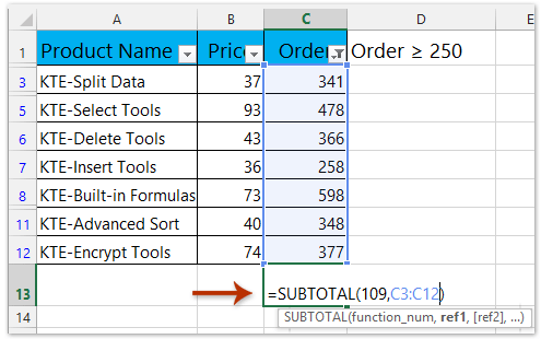
Excel formula to sum only visible cells. That way adding more data will automatically update the formula results. If your data from A2 to A20. 3 Building a Total Row.
A SUBTOTAL formula will be inserted summing only the visible cells in the column. And then the summing result is calculated with ignoring all hidden cells. It does this by multiplying each cell in the Sales column by the corresponding cell in the Visible column then summing the result.
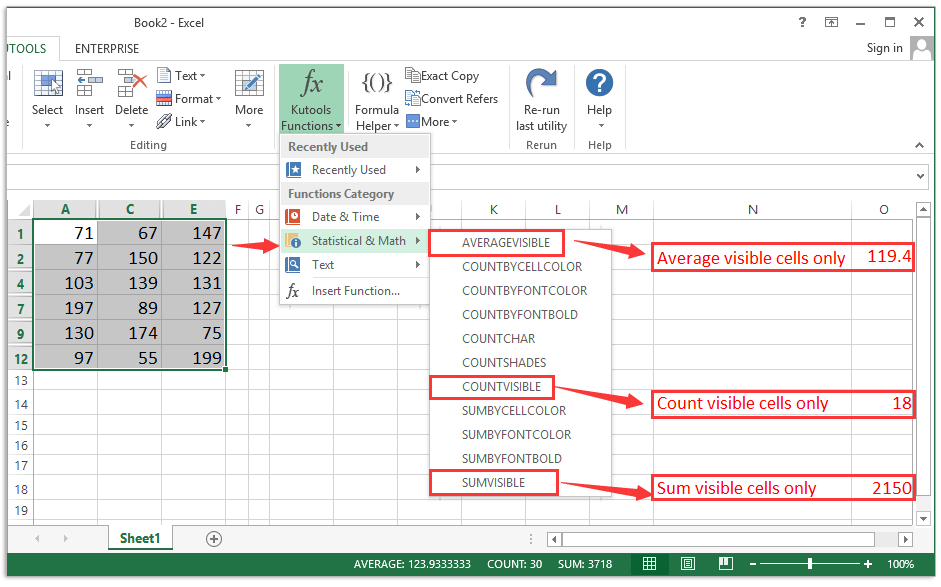
SUMPRODUCTcriteriarange criteria0SUBTOTAL109OFFSETsumrangeROWsumrange-MINROWsumrange011 The first part criteriarange criteria0 just checks the. Above all we need to find a proper function can only sum visible cells in a filtered list and ignore the filtered-out data. With Kutools for Excel you also can count or calculate the average in visible cellsrowcolumns.
If youve happened to read the COUNTIF tutorial on this blog you wont have any difficulties with understanding Excel SUMIF because its syntax and usage is analogous. Heres the first formula that relies on the Visible column. You can select one of the calculation types from a in-cell drop-down menu in the Totals Row and the SUBTOTAL function will automatically be created for you.
Sum visible columns only. Generically to sum sumrange based on a match in criteriarangebut only for visible. If we need to SUM visible columns only we will need a twist.
In this case 109 sums all visible cells in a cell range. SUBTOTAL 109C3C12 The first argument allows you to pick a function number that determines how the SUBTOTAL function behaves. Just organize your data in table Ctrl T or filter the data the way you want by clicking the Filter button.
5 back to the current worksheet then type the following formula in a blank cell. The formula used is. The twist is not difficult at all.
Works only in vertical direction not horizontal. It is best to use it with Excel Tables as shown above. In other cases you can use Excel macros.
Actually excel built-in SUBTOTAL function can perform calculating like sum data count average for both visible invisible cells or only visible cells. It doesnt matter if hidden are rows or columns. Excel Tables also use the SUBTOTAL function in the Totals Row of a Table.
The below formula will help to sum the visible rows in a filtered list. In A1 input the formula. How to SUM Only Visible or Filtered Rows Using SUBTOTAL.
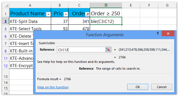
Function SumVisibleCRange As Object ApplicationVolatile TotalSum 0 For Each cell In CRange If cellColumnsHidden False Then. For example you want to sum only visible cells only please select the cell you will place the summing result at type the formula SUMVISIBLEC3C12 C3C13 is the range where you will sum only visible cells into it and press the Enter key. CELLwidthA1 copy across to F1.
However there is no similar function for visible columns only. Sum values based on first occurrence of other column using excel formula with Subtotal function 1 Excel OFFSET function to work on visible cell only Formula to generate summary title for repeated cells. What we need is a helper row say Row 1 in our example and SUMIF function.
You will be surprised at the function that saves the day. Here is a VBA function that do SUM for visible cells only. In the example shown a filter has been applied to the data and the goal is to sum the values in column F that are still visible.
Please Login or Register to view this content. In this case 109 sums all visible cells in a cell range. 6 Download the SUBTOTAL Example File.
How to use a SUMIF to sum the visible cells that match a criteria. If my answer or that of other members has helped you please say Thanks by clicking the Add Reputation button at. To hide a value simply right click on a row number and then click on Hide to.
The SUMIF function also known as Excel conditional sum is used to add cells based on a certain condition or criteria. 1 Examine the Data Set. 2 Creating a Data Table.
To sum only the visible rows use the SUBTOTAL function with function number 9 or 109. 5 Using SUBTOTAL to SUM a Filtered Table. Works from Office 2010 onwards.
Learn how to Sum visible cells only using the Aggregate function. Generically to sum sumrange based on a match in criteriarangebut only for visible rows you can use this formula. The SUBTOTAL function will return the results of the visible cells only.
SUMPRODUCT Table1 Sales Table1 Visible1 This formula uses the SUMPRODUCT to return the sum of the visible rows in Table1. In the Function Arguments dialog click to select cells you want to sum into the Reference textbox and you can preview the calculated result at the bottom. 4 Filtering Data Table Rows.
Click OK and only the visible columns have been summed. The usual SUM function wont work in this case you need the SUBTOTAL function. After that select the cell immediately below the column you want to total and click the AutoSum button on the ribbon.

How To Sum Only Filtered Or Visible Cells In Excel

Excel Formula Sum Visible Rows In A Filtered List Exceljet
How To Sum Only Filtered Or Visible Cells In Excel
How To Sum Only Filtered Or Visible Cells In Excel

Sum Of Positive And Negative Numbers From Column Sumif Function Excel Formula Excel Function Excel Formula Positive Numbers Negative Numbers
How To Sum Only Filtered Or Visible Cells In Excel

See How To Sum In Excel Using The Autosum Feature And How To Write Your Own Sum Formula In Excel To Total A Column Rows Or Selected Range Le Excel Column

Use The Subtotal Feature In Excel For A Variety Of Calculations Excel Excel Tutorials Excel Hacks

Excel Formula Remove Leading And Trailing Spaces From Text Excel Formula How To Remove Excel Hacks

Tidak ada komentar:
Posting Komentar