Excel Formula Vlookup If Then

If you have to find out what are the names that are in column B that not there in column A you can use the below VLOOKUP formula. Let us have a look at how to use VLOOKUP from another sheet and then how it can be used on another workbook.

Excel Dan Rumus Microsoft Excel Rumus Excel If Vlookup

One of these functions is.

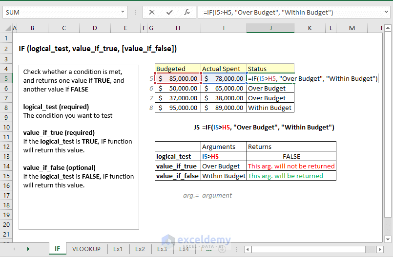
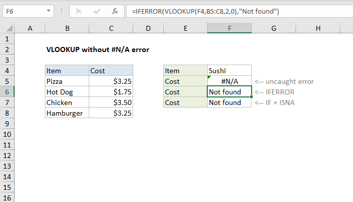
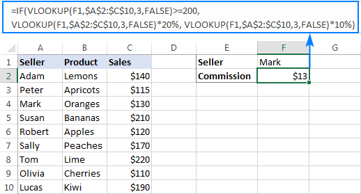
Excel formula vlookup if then. IFERROR VLOOKUP B2Lookup tableA2B5 2 FALSE As you can see it returns nothing when the lookup value is not in the search list. When we use the IF function with Vlookup then the IF statement compares the result obtained from the vlookup statement with the selected value. In our example the formula goes as follows.

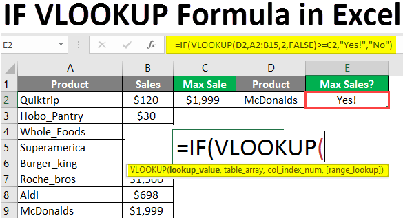
Introduction to VLOOKUP Formula in Excel Using Vlookup along with IF Function in Excel is used to get conditional results on the basis of compared values. The IF function checks if the value in cell F2 is Shop 1 or 2. 33 rows VLOOKUP B2C2E73TRUE In this example B2 is the first argument an.

Formula-free way to do vlookup in Excel. A generic formula to Vlookup across sheets is as follows. Besides you can vlookup and get the adjacent cell value based on a cell reference.

Select the result cell and then drag the Fill Handle to apply the formula to other cells In this case I drag the Fill Handle down until it reaches B18. This method requires a little preparation but in the end you will have a more compact formula to Vlookup in any number of spreadsheets. To return zero instead of NA when the VLOOKUP function cannot find the correct relative result you just need to change the ordinary formula to another one in Excel.

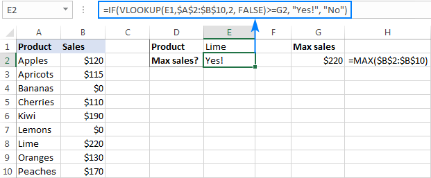
Below you will a find a few real-life uses of this IF Vlookup formula. IF VLOOKUP sample_value TRUE FALSE Translated in plain English the formula instructs Excel to return True if Vlookup is true ie. VLOOKUPMAXA2A11 A2B11 2 FALSE Then the adjacent cell value of the largest weight in column A is populated in the selected cell.

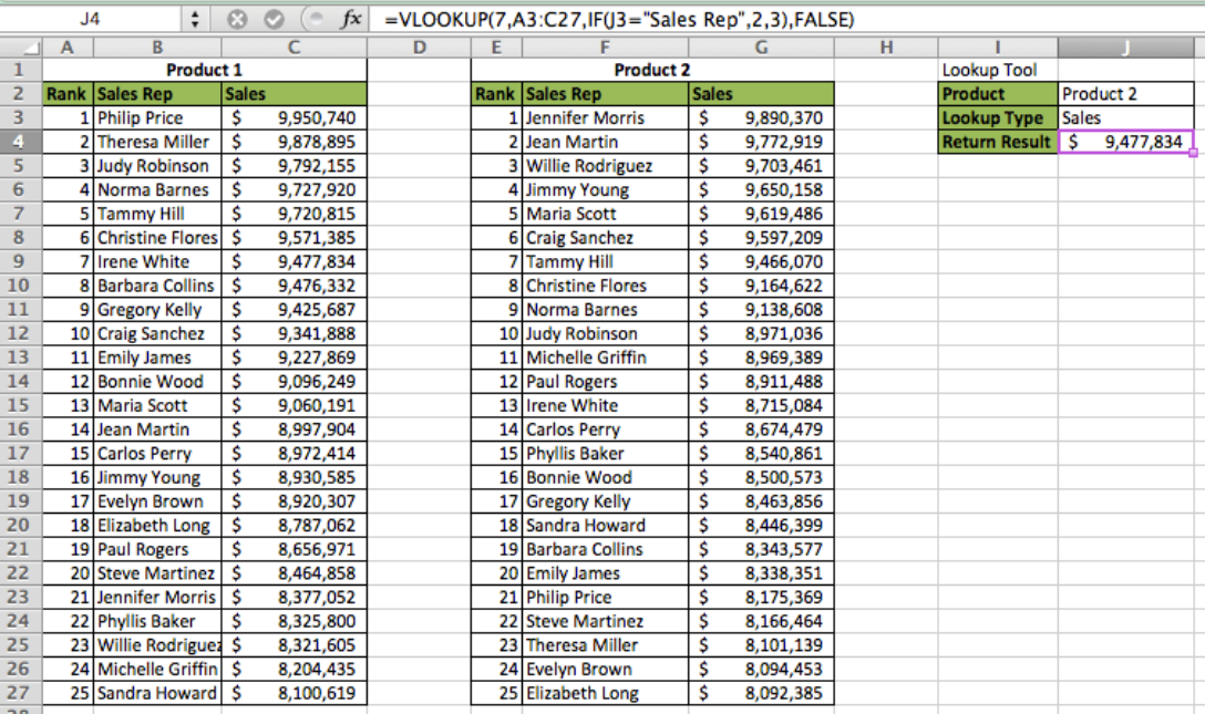
IFISERRORVLOOKUPB2A2A1010Not AvailableAvailable The above formula checks the name. Select the result cell and then drag the Fill Handle to apply the formula to other cells In this case I drag the Fill Handle down until it reaches B18. In cell J4 type this formula.

According to this condition the VLOOKUP then returns the corresponding price for the product. If youd like to replace the error with. If the result from VLOOKUP is an empty string return an empty string.

Equal to the sample value. Excel has several very effective functions when it comes to lookup values in other columns. Probably for beginners level you must have practiced the formula from the same sheet itself.

For our sample dataset the formula goes as follows. The VLOOKUP function allows us to lookup a specified value within a column of data and then return a value adjacent to the matching value. Fetching the data from another worksheet or from another workbook is slightly different using the VLOOKUP function in excel.

IFVLOOKUP sample_value TRUE FALSE Typical use cases for these include. Compare the value returned by Vlookup with that of a sample value and return TrueFalse YesNo or 1 out of 2 values determined by us. IF ISNA VLOOKUP A2D2D41FALSE No Yes 3.

Enter the below formula into it and press the Enter key. SUMIFMain_tableID VLOOKUPF2 Lookup_table 2 FALSE Main_tableSales Download this VLOOKUP and SUMIF sample. In a similar manner you can do multiple Vlookup with three four or more conditions.

If Vlookup is false not equal to the sample value the formula returns False. LOOKUPLookup Value Table Array Return Column Approximate Match TRUEFALSE Type the number 7 in cell J3. The generic formula will be.

One more way to Vlookup between multiple sheets in Excel is to use a combination of VLOOKUP and INDIRECT functions. Now all you need is to assemble the formulas parts and your SUMIF VLOOKUP formula is ready. Select a blank cell here I select cell C3 enter the below formula into it and then press the Enter key.

To return zero instead of NA when the VLOOKUP function cannot find the correct relative result you just need to change the ordinary formula to another one in Excel. Applying the VLOOKUP Formula. Select the cell you want to use VLOOKUP function and type this formula IFERROR VLOOKUP A13A2C10300 drag the autofill handle to the range you need.

IFERROR INDEX C3C30 SMALL IF 1 -- E3A3A30 -- F3B3B30 ROW C3C30-2 COLUMN -6 And the result can resemble this. To test the result of VLOOKUP directly we use the IF function like this.

Examples Of Vlookup With The If Condition Excelchat