

Sometimes your specified data is not in the data range to get the nearest match with the given data you need to use the vlookup to get an approximate match. In case of Approximate Match typeIn case of approximate match type TRUE your VLOOKUP function generates NA error if your lookup value is smaller than the smallest value available in the first column of table_array.
Using Vlookup With If Condition In Excel 5 Examples Exceldemy
If your laptop doesnt offer a number keypad you could use SUBSTITUTED2CHAR160 in column E.
Excel formula if vlookup not match. Instead well use the MATCH function to find Chicago in the range B1B11. In most cases people are looking for a particular product order employee or customer and therefore require an exact match. If you are working on multiple column data its a pain to change its reference because you have to do this manually.
How to Use VLookup and Match formulas in Excel In this article we will learn how to use ISERROR function along with Vlookup function to ignore the error as result in Microsoft Excel. IFVLOOKUPA1 data col0 VLOOKUPA1 data col0. Use vlookup function to get the approximate matches in Excel.
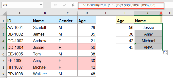
Below is the IF formula that returns Match when the two cells have the cell value and Not a Match when the value is different. In VLOOKUP col_index_no is a static value which is the reason VLOOKUP doesnt work like a dynamic function. VLOOKUP Not Detecting Text Matches.
Select the result cell and then drag the Fill Handle to apply the formula to other cells In this case I drag the Fill Handle down until it reaches B18. Enter the formula and then Paste Values to column D to replace the nonbreaking spaces with regular spaces. Now if your spreadsheet isnt built this way then do not use VLOOKUP.
The last argument of the VLOOKUP function known as range_lookup asks if you would like an approximate or an exact match. Generally if you enter wrong data type in the formula in Excel then formula generates Value error. Use the combination of INDEX and MATCH functions instead.
This example shows a small list where the value we want to search on Chicago isnt in the leftmost column. When looking for a unique value FALSE should be entered for the range_lookup argument. If match_type is 0 and lookup_value is text the wildcard characters question mark and asterisk can be used in lookup_value.
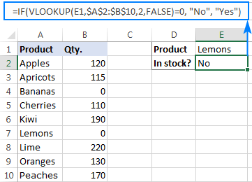
The best way to solve this problem is to use MATCH Function in VLOOKUP for col_index_number. If you are sure the relevant data exists in your spreadsheet and VLOOKUP is not catching it take time to verify that the referenced cells dont have hidden spaces or non-printing characters. IFISNAVLOOKUPA2D2D41FALSE No Yes 3.
If we merge the VLOOKUP and MATCH functions together we can create our own custom formula which will work as a two-way lookup formula that enables us to easily cross check. Also ensure that the cells follow the correct. The MATCH formulas will start to work.
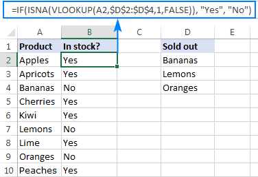
So we cant use VLOOKUP. Here is my formula. To compare each cell in the target column with another list and return True or Yes if a match is found False or No otherwise use this generic IF ISNA VLOOKUP formula.
Enter the below formula into it and press the Enter key. Match returns the NA error if no match is found The argument lookup_array must be placed in descending order. IF A2B2MatchNot a Match The above formula uses the same condition to check whether the two cells in.
Use the TRIM formula on both corresponding columns and then remove formulas to make sure all cells in both corresponding columns are text fields. The description Approximate Match would tend to imply that the function would match ABC Company and ABC Company Inc since they are approximately the same name. Or carefully copy the nonbreaking space from a cell in column D and paste that.
All or some of the cells in either of the corresponding columns arent being recognized as a Text fieldcell. How can I change it to return 0 instead of NA if there is not a match for A2 on the look up table q4_03. Click the Replace All button.
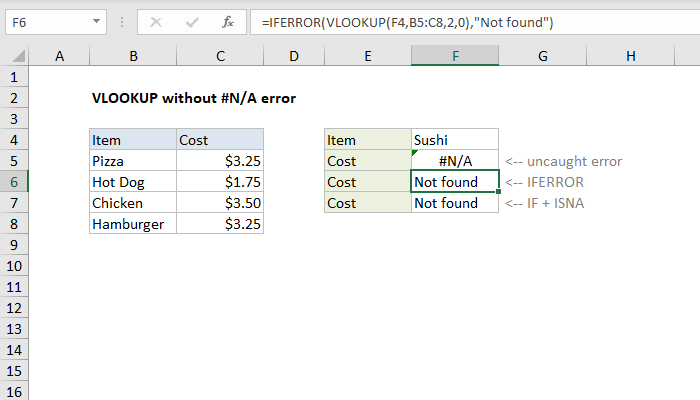
When the range_lookup argument is FALSEand VLOOKUP is unable to find an exact match in your datait returns the NA error. When you select TRUE Approximate Match you are not asking Excel to match values that are approximately the same as each other. TRUE FALSE Z-A2 1 0 -1 -2 and so on.
How To Vlookup Values From Right To Left In Excel
Excel Formula Faster Vlookup With 2 Vlookups Exceljet

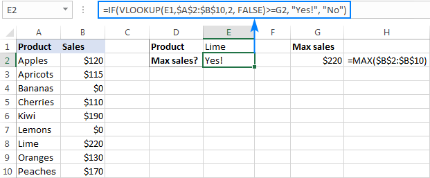
If Vlookup In Excel Vlookup Formula With If Condition
If Vlookup In Excel Vlookup Formula With If Condition
Excel Formula Vlookup Without N A Error Exceljet
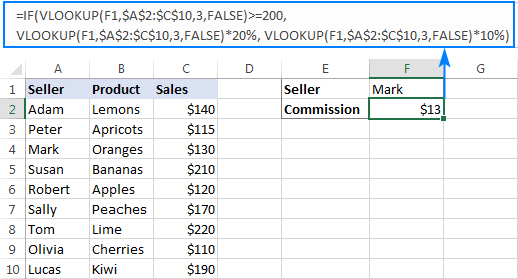
If Vlookup In Excel Vlookup Formula With If Condition
How To Vlookup To Return Blank Or Specific Value Instead Of 0 Or N A In Excel
Use Iferror With Vlookup To Get Rid Of N A Errors

If Vlookup In Excel Vlookup Formula With If Condition

Tidak ada komentar:
Posting Komentar